In this articles we’re going to implement a Mark-Sweep garbage collector in C++.
This is the 9th lecture from the Essentials of Garbage Collectors course where we discuss in detail all the aspects of automatic memory management.
Audience: advanced engineers
By itself the “garbage collection” topic relates to abstract algorithms of collecting the data which isn’t used anymore (the “garbage”). For example, it might be a collection of objects in some array, records in a database, nodes in a graph, etc. The main use-case though for garbage collectors are runtime systems in programming languages.
Prerequisites for this lecture are the:
- Lecture 3: Object header
- Lecture 4: Virtual Memory and Memory Layout
- Lecture 7: Tracing vs. Direct collectors
Video lecture
Before going to the lab session, you can address corresponding video lecture on Mark-Sweep collector from the class:
Lecture 9/17: Mark-Sweep collector
Let’s start from discussion about tracing and direct collectors.
Tracing vs. Direct collectors
As we know from the lecture 7, all GC algorithms are divided into tracing and direct.
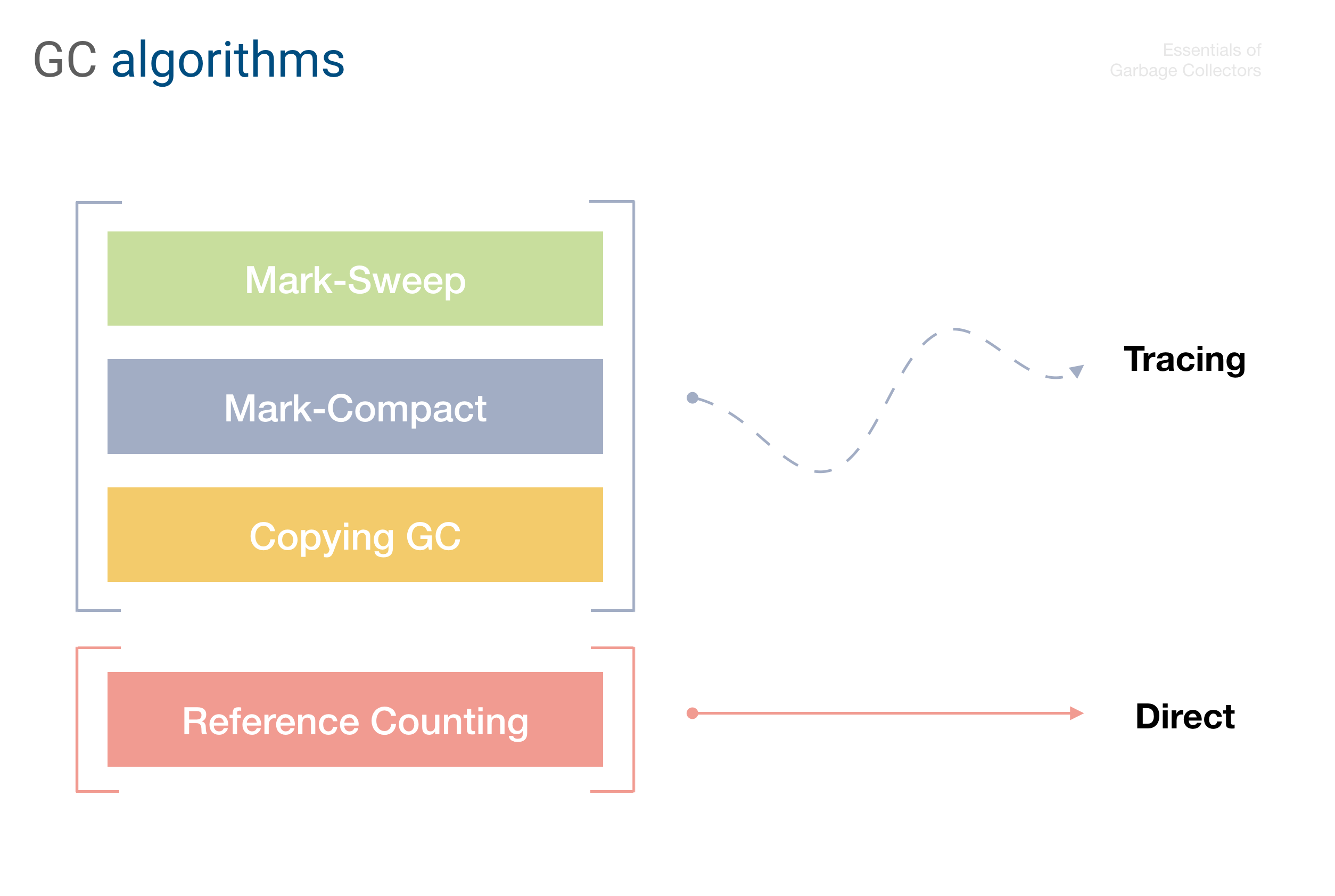
Tracing vs. Direct collectors
And despite being called “garbage” collectors, the tracing collectors actually do not identify the garbage. Instead it’s quite the opposite — they identify alive objects, treating by extension everything else as a garbage.
Mark-Sweep is a tracing collector, so we’re going to have the tracing stage in our implementation.
Mark-Sweep example
Note: C++ also has a trivial Reference Counting collector in the view of std::shared_ptr.
Since we chose implementing the collector in C++, we shall now discuss some specifics related to its runtime system.
C++ specifics
Below are some details related to C++ runtime, which affect our implementation.
Exposed pointers semantics
As we’ve been discussing during this class, C++ exposes the pointer semantics to user-level. This means, we can obtain a pointer to an object, and store it as an observable value, in some variable.
This in turn makes implementing a moving (like Mark-Compact) or copying (Generational, Semi-Space collectors) much harder in C++ runtime: if we relocate an object, all the pointers will be invalidated, and contain incorrect addresses.
For languages like Java, JavaScript and others, which do not work with raw memory directly in user-code, it is much simpler, with many other options.
Luckily, Mark-Sweep is a non-moving collector, which means we can implement it in C++, and what is quite an interesting engineering task, since we’ll need to touch concepts of the stack, registers, a bit of Assembly, and others things.
Pointer or number?
To implement the tracing algorithm we should be able to obtain all (child) pointers inside an object’s shape. Then to follow the child pointers, and obtain their pointers again, etc — traversing the whole object graph.
However, once we obtained a pointer in C++, in general we can’t tell whether it’s really a pointer, or just a simple number — recall, a garbage collector works at lower-level where there are only bytes, but not actual concrete C++ structures.
Again, managed high-level languages, such as Java, JS, etc. keep track of value types and can easily distinguish a pointer from other values. For this such languages use different types of value encoding, the most popular of which are the Tagged pointers and NaN-boxing. The encoding always assume inverse operation of decoding, which usually happens at runtime. It may slow down the operations, but it’s a de-facto standard for implementing most of the dynamic programming languages.
In C++ instead of encoding the values (and constantly decoding them at runtime), we’re going to use a conservative approach with a “duck test” — if it looks like a pointer, and really points to a known heap address, then it must be a pointer, and we need to trace it. Not surprisingly such collectors are exactly called as conservative.
GC roots
The garbage collector root objects (or simply, roots) are the starting point from which we begin our trace analysis. These objects are guaranteed to be alive, since usually are pointed by the global or local variables on the stack.
Higher-level virtual machines may track all the roots for GC purposes, making procedures such as getRoots much simpler. However in C++ we’ll have to manually traverse the stack, collecting conservatively the roots.
In addition, some of the local variables may be placed in CPU registers, and we’ll have to traverse those too. Luckily, we can use a trick of pushing all the registers onto the stack, which we’ll save us some time and implementation effort.
OK, let’s now dive directly into the implementation, and will start from the object graph.
Implementation
We’re going to use top-down approach in this implementation, starting from the high-level and essentials concepts, leaving C++ specific details to the end.
Traceable objects
The crucial part of our implementation will be the Traceable object, which would track all the needed information for the garbage collector’s purposes. We will describe the details of the Traceable struct a bit later, and for now let’s just show how we can create structs which simply inherit it:
/**
 * Traceable Node structure.
 *
 * Contains the name of the node, and the
 * pointers to left and right sub-nodes,
 * forming a tree.
 */
struct Node : public Traceable {
  char name;

  Node *left;
  Node *right;
};
All traceable objects have access to so-called Object header, which contains the GC meta-information. Let’s see what it is.
Object header
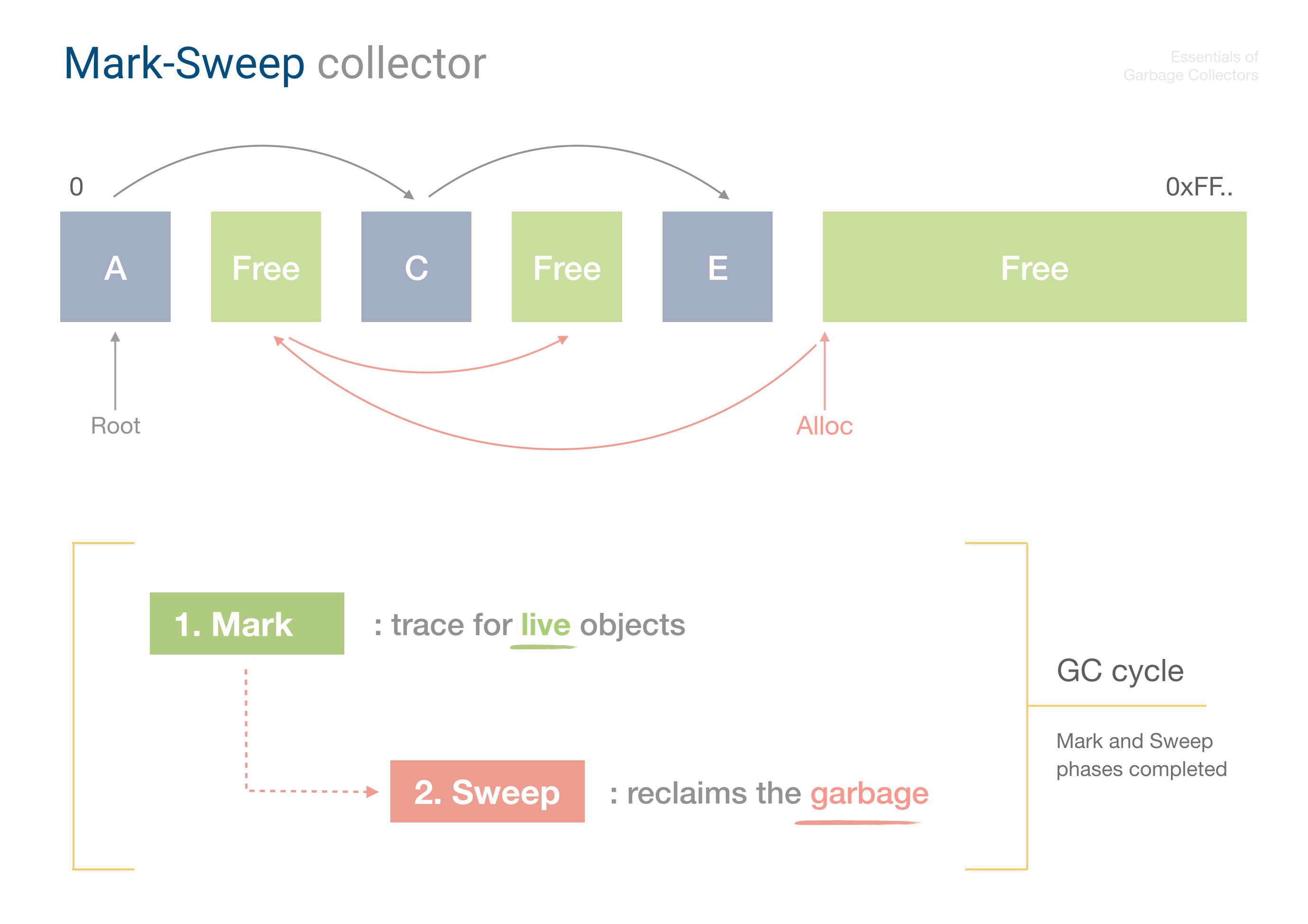
The Mark-Sweep collector as the name assumes consists of two phases: Marking phase (the trace for alive object), and Sweeping phase (garbage reclaim). To mark the objects as alive, the collector needs to store this flag somewhere, and this is where object header comes into play.
Our header will contain two fields: the mark-bit, and the size of the object:
/**
 * Object header.
 */
struct ObjectHeader {
  bool marked;
  size_t size;
};
And each traceable object gets access to its header (via the base Traceable class):
// Create a node:
auto node = new Node {.name = 'A'};

// Obtain the header:
auto header = node->getHeader();

std::cout << header->marked; // false
std::cout << header->size; // 24
User-code in general doesn’t need to (and shouldn’t) access the header meta-information, and this is mainly for GC itself. However we expose it here as a public method for educational purposes.
OK, now when we have ability to create objects with traceable meta-info, let’s create our working graph.
Object graph
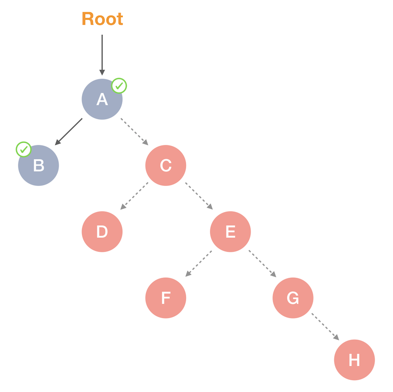
Here’s the example of the object graph, which we’ll be using in further analysis:
/*

   Graph:

     A        -- Root
    / \
   B   C
      / \
     D   E
        / \
       F   G
            \
             H

*/

Node *createGraph() {
  auto H = new Node{.name = 'H'};

  auto G = new Node{.name = 'G', .right = H};
  auto F = new Node{.name = 'F'};

  auto E = new Node{.name = 'E', .left = F, .right = G};
  auto D = new Node{.name = 'D'};

  auto C = new Node{.name = 'C', .left = D, .right = E};
  auto B = new Node{.name = 'B'};

  auto A = new Node{.name = 'A', .left = B, .right = C};

  return A;  // Root
}
Then we create this object graph in our main function, having only the object A as a root:
int main(int argc, char const *argv[]) {
  gcInit();                                 // (1)

  auto A = createGraph();                   // (2)

  // Full alive graph:
  dump("Allocated graph:");                 // (3)

  ...

  return 0;
}
Notice how in (1) we call gcInit() function — before any operation related to traceable objects allocation. We will discuss this function a bit later, and for now let’s take a look at our graph picture, which we create at (2):
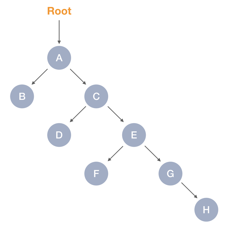
Allocated object graph
So it’s a tree, created by nodes, with left- and right-hand sides in each node. Currently as we see, only the variable A is guaranteed to be a known reachable reference. And in general we don’t know anything else yet about the sub-nodes of A — since none of them are pointed by variables.
In (3) we dump the allocated heap, which shows us the addresses and the object headers of each object:
------------------------------------------------
Allocated graph:

{
  [H] 0x7fed26401770: {.marked = 0, .size = 24},
  [G] 0x7fed264017d0: {.marked = 0, .size = 24},
  [F] 0x7fed26401830: {.marked = 0, .size = 24},
  [E] 0x7fed26401890: {.marked = 0, .size = 24},
  [D] 0x7fed264018f0: {.marked = 0, .size = 24},
  [C] 0x7fed26401950: {.marked = 0, .size = 24},
  [B] 0x7fed264019b0: {.marked = 0, .size = 24},
  [A] 0x7fed26401a10: {.marked = 0, .size = 24},
}
As we can see, none of them are marked yet, since GC cycle wasn’t executed yet. Also, none of them are garbage yet.
We shall discuss now how this garbage may appear in our memory.
The garbage
How does the “garbage” appear in our memory, and what is the “garbage” anyways?
From a tracing collector perspective, a garbage is an unreachable object. This basically means the object wasn’t visited during the tracing phase.
Note: in contrast with the Reference Counting collector which analyses the number of references to an object, the tracing collectors use concept of reachability: an object may still have a reference to it, but at the same time be an unreachable garbage.
Let’s see it in action:
// Detach the whole right sub-tree:
A->right = nullptr;
This single operation basically turns into a garbage the whole right sub-tree of the object A. Slight correction: it’s the garbage in a garbage-collected system; in pure C++ this actually would be a memory leak.
Clearly, only the left sub-tree is reachable at this point, and everything else is a garbage:
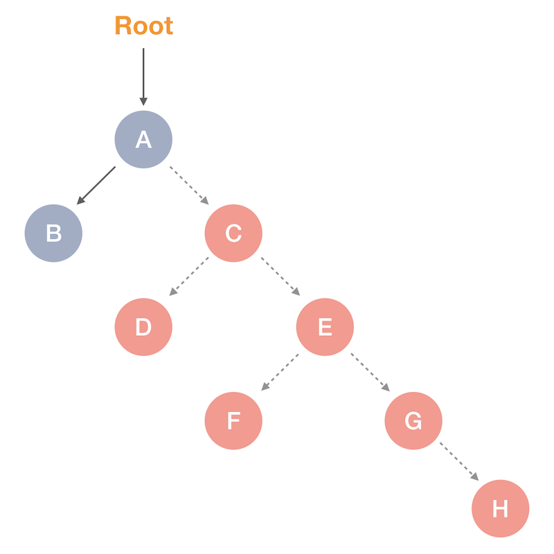
Reachable vs. Garbage objects
Now it is a good time to go deeper into the implementation, and see what happens inside the GC-cycle of our program.
Custom allocator
In the lecture 6 devoted to implementing a Memory Allocator, we’ve been discussing how to build a custom allocator, similar to malloc function.
Here we’ll be using specific C++ feature, overriding the default behavior of the new operator. By itself this operator is a thin-wrapper on top of the default malloc allocator. Our implementation will also be a thin-wrapper which initializes the object header for our data.
This is done in the base Traceable class which we’ve been discussing above:
/**
 * The `Traceable` struct is used as a base class
 * for any object which should be managed by GC.
 */
struct Traceable {
  ObjectHeader *getHeader() { return traceInfo.at(this); }

  static void *operator new(size_t size) {
    // Allocate a block:
    void *object = ::operator new(size);

    // Create an object header for it:
    auto header = new ObjectHeader{.marked = false, .size = size};
    traceInfo.insert(std::make_pair((Traceable *)object, header));

    // Result is the actual block:
    return object;
  }
};
Here we allocate the object header, and store it in the extra traceInfo data structure, which is a map from the allocated pointer to its header.
Note: alternatively the object header is co-located with the payload pointer.
Finally let’s go down to the actual collection algorithm.
Mark phase
Let’s start from the code for of our main function again, to see how we call the GC cycle:
int main(int argc, char const *argv[]) {
  gcInit();

  auto A = createGraph();

  // Full alive graph:
  dump("Allocated graph:");

  // Detach the whole right sub-tree:
  A->right = nullptr;

  // Run GC:
  gc();

  return 0;
}
And our gc function will also be trivial — calling the mark phase, followed by the sweep phase:
/**
 * Mark-Sweep GC.
 */
void gc() {
  mark();
  dump("After mark:");

  sweep();
  dump("After sweep:");
}
After each step we dump the heap to see how the data is changed. Let’s start from the mark phase, and see the results.
If you followed the video lecture, this code should already be familiar to you:
/**
 * Mark phase.
 */
void mark() {
  auto worklist = getRoots();

  while (!worklist.empty()) {
    auto o = worklist.back();
    worklist.pop_back();
    auto header = o->getHeader();

    if (!header->marked) {
      header->marked = true;
      for (const auto &p : getPointers(o)) {
        worklist.push_back(p);
      }
    }
  }
}
To reiterate, we start our analysis from the roots, initializing the worklist. Going through each object in this work list, we mark it as alive, and then go deeper to the child pointers, also adding them to the working list.
By the end of this operation, the whole visited graph will be marked as alive. The unvisited objects will eventually be reclaimed being a garbage. For this we’ll need to implement the getRoots and getPointers functions used above.
After this traversal, our graph looks as follows:
Marked alive objects
And what is reflected in our memory dump:
------------------------------------------------
After mark:

{
  [H] 0x7fed26401770: {.marked = 0, .size = 24},
  [G] 0x7fed264017d0: {.marked = 0, .size = 24},
  [F] 0x7fed26401830: {.marked = 0, .size = 24},
  [E] 0x7fed26401890: {.marked = 0, .size = 24},
  [D] 0x7fed264018f0: {.marked = 0, .size = 24},
  [C] 0x7fed26401950: {.marked = 0, .size = 24},
  [B] 0x7fed264019b0: {.marked = 1, .size = 24},
  [A] 0x7fed26401a10: {.marked = 1, .size = 24},
}
Marking doesn’t reclaim the garbage, it only identifies the alive objects. And this is relatively a fast cycle — we visit only a small sub-set of the alive data. In contrast, the sweep phase has to traverse the whole heap. Let’s take a look.
Sweep phase
Since we track all the allocated objects in our traceInfo data structure, the sweep phase can leverage it for traversal:
/**
 * Sweep phase.
 */
void sweep() {
  auto it = traceInfo.cbegin();
  while (it != traceInfo.cend()) {
    if (it->second->marked) {        // (1)
      it->second->marked = false;
      ++it;
    } else {
      it = traceInfo.erase(it);
      delete it->first;              // (2)
    }
  }
}
So here in (1) we check if an object is alive, that is, its mark-bit is set. In this case we reset the mark-bit (for the future collection cycles), and proceed further, keeping the object on the heap.
Otherwise, the object wasn’t visited during the trace, and it means it’s a garbage, so in (2) we immediately reclaim it.
After the sweep phase our heap looks as follows:
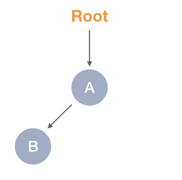
Reclaimed garbage
This is also reflected in our heap dump — the whole right sub-tree is gone:
------------------------------------------------
After sweep:

{
  [B] 0x7fed264019b0: {.marked = 0, .size = 24},
  [A] 0x7fed26401a10: {.marked = 0, .size = 24},
}
And this is basically the whole algorithm!
Now when we know how it works, let’s finally take a deeper look at specific C++ details of obtaining the pointers and the roots.
Obtaining pointers
In the mark phase above we used the getPointers helper function which returns the child pointers of an object.
Let’s take a look at the implementation:
/**
 * Go through object fields, and see if we have any
 * which are recorded in the `traceInfo`.
 */
std::vector<Traceable *> getPointers(Traceable *object) {
  auto p = (uint8_t *)object;
  auto end = (p + object->getHeader()->size);
  std::vector<Traceable *> result;
  while (p < end) {
    auto address = (Traceable *)*(uintptr_t *)p;
    if (traceInfo.count(address) != 0) {
      result.emplace_back(address);
    }
    p++;
  }
  return result;
}
The idea here is we go through each field, and see if any “looks like a pointer”, and whether it’s recorded in our known heap addresses. If yes, we conservatively treat it as a pointer. Here’s also when we come to our size field from the object header. I’m leaving the check for false-positive pointers for you as an assignment.
OK, now when we can obtain the child pointers, let’s see at how we get the roots.
Determining roots
Warning: this part is very C++ specific and is low-level. In general, the following implementation details can be skipped and are not required for understanding the Mark-Sweep algorithm itself. Proceed only on your interest.
A root, as we know, is a reachable alive reference, which usually is represented by a variable or a register. For this we’ll need to scan the current stack (in general, all stacks from active threads), and see whether some variables are stored in registers.
For this we introduce the procedures for reading frame and stack pointers:
/**
 * Frame pointer.
 */
intptr_t *__rbp;

/**
 * Stack pointer.
 */
intptr_t *__rsp;

#define __READ_RBP() __asm__ volatile("movq %%rbp, %0" : "=r"(__rbp))
#define __READ_RSP() __asm__ volatile("movq %%rsp, %0" : "=r"(__rsp))
In addition our gcInit called from main initializes the main frame address — this will be our stop border in stack traversal:
/**
 * Main frame stack begin.
 */
intptr_t *__stackBegin;

/**
 * Initializes address of the main frame.
 */
void gcInit() {
  // `main` frame pointer:
  __READ_RBP();
  __stackBegin = (intptr_t *)*__rbp;
}
Note: alternatively one can use non-standard __builtin_frame_address function to obtain main frame address.
Finally here’s our getRoots function:
/**
 * Traverses the stacks to obtain the roots.
 */
std::vector<Traceable *> getRoots() {
  std::vector<Traceable *> result;

  // Some local variables (roots) can be stored in registers.
  // Use `setjmp` to push them all onto the stack.
  jmp_buf jb;
  setjmp(jb);

  __READ_RSP();
  auto rsp = (uint8_t *)__rsp;
  auto top = (uint8_t *)__stackBegin;

  while (rsp < top) {
    auto address = (Traceable *)*(uintptr_t *)rsp;
    if (traceInfo.count(address) != 0) {
      result.emplace_back(address);
    }
    rsp++;
  }

  return result;
}
Here we traverse the stack, reading the current %rsp, and go until we hit the top point, which is set to the __stackBegin.
Note: you may also need to use __attribute__((noinline)) for particular functions to preserve the stack frames.
Notice the trick we use with the setjmp. To make it simpler, and avoid manually messing with the registers, we just push them all onto the current frame. If any traceable object is in a register, our getRoots analysis will be able to find it, traversing only the stack.
At this point we may consider our implementation completed.
Conclusion
I hope this lecture clarified some details of the Mark-Sweep garbage collector, and showed specifics of implementing it in a lower-level language, which exposes the pointers semantics. Implementing the Mark-Sweep in a virtual machine with predictable value types, and which hides all the details of stack frames, registers, and pointers, at this point should be much simpler.
There are many other improvements to the basic implementation we showed here, for example, collecting per generation, or using Concurrent Mark-Sweep (CMS) implementation.
In addition, the Mark-Sweep being a non-moving collector, has an issue of heap fragmentation, since the allocator should reuse the reclaimed objects keeping them in-place. Mark-Compact and Copying collectors, which we discuss in the following lectures 10 and 11, fix this issue.
You can find the full source code for this lecture in this gist.
If you got interested and would like to follow this course, you can always enroll here:
Thanks, and see you in the class!
nice write-up, thanks!
can you clarify please how we get main frame address?
@jeremy chen, as mentioned in the note, you can also use the __builtin_frame_address:
I used instead raw reading from
%rbpregister:The
%rbppoints to the current frame, so dereferencing it gives us the parent, that ismain, frame.What application did you use to draw your charts ?
Write up is simple! But why did you use a tree to represent object connections? It will usually look like a directed graph right?
@Sheera Shamsu thanks! A tree is a graph 😉
Thanks for such a good article. But I noticed a strange behavior, if you call gc () 2 times in a row, then the name of one of the nodes is sometimes distorted. I tracked that this happens after adding an element to the vector in the getRoots () function. Any idea why this might be?
hi i have a question about how getRoots() work, isn’t it actually unsafe to read data from stack frames and trying to see if the pointer is in the traceinfo vector? i’m asking this because i think it could be possible to read a long x = some_random_value; and assuming it’s a pointer just because its value is equal to a pointer allocated somewhere else
@christallo – good point, and this shows that dealing with untagged values might be hard. That’s why the CG is called conservative, and most of the managed languages and VMs use a type tag to distinguish actual values, and implementing a GC module is much simpler there. We show the generic idea here, and you can extend it further.
Hello, I have a question regarding getRoots(), in the function the registers are first pushed to the stack and then %rsp is read, but since rsp is incremented in the loop, wouldn’t that mean that the register that were pushed to the stack are never scanned? Since rsp points to the stack top(meaning just after the jb we pushed onto the stack)
Great tutorial!
@Andrea, in this architecture (and usually) the stack grows downwards, so increasing the stack pointer means we actually go backwards in all stack frames, until we reach the main frame. So the pushed registers should be met.
I think these two lines need to be swapped:
“`
it = traceInfo.erase(it);
delete it->first;
“`
Because erase method returns the [“iterator following the last removed element”](https://en.cppreference.com/w/cpp/container/map/erase).
I made a few changes for this to run on M1 macOS: https://gist.github.com/agentcooper/425c7eec022fa806f4db537c171cba70. It is also possible to use the leaks utility bundled with Xcode to verify that there are indeed no leaks, see my comment under the GitHub Gist.
Hello! Thank you for sharing your knowledge with others, this is very valuable!
In windows for some reason I can not get the roots, it is always returning 0 roots. Here is my assembly code to get the rsp and rbp pointers:
.asm
; File: read_rbp.asm

.code
PUBLIC read_rbp

read_rbp PROC
    mov rax, rbp    ; Move the value of rbp into rax
    mov [rcx], rax  ; Store the value of rbp at the address in rcx (first argument in x64 calling convention)
    ret
read_rbp ENDP

PUBLIC read_rsp

read_rsp PROC
    mov rax, rsp    ; Move the value of rsp into rax
    mov [rcx], rax  ; Store the value of rsp at the address in rcx (first argument in x64 calling convention)
    ret
read_rsp ENDP

END

.cpp
extern "C" uintptr_t read_rbp(intptr_t**);
extern "C" uintptr_t read_rsp(intptr_t**);
#define __READ_RBP() read_rbp(&__rbp)
#define __READ_RSP() read_rsp(&__rsp)
I hope you can help me, thank you very much!
It does not work in Windows 64 bit for me. Had to add a separate asm for the functions, but still not working. Which platform and OS did you use? Thank you